逻辑回归

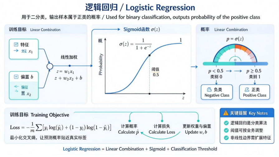
逻辑回归属于监督学习分类算法，多用于二分类任务。虽然名字带“回归”，但它不预测连续数值，而是预测样本属于某一类别的概率。

1. 基本原理

逻辑回归先做线性计算，再送入Sigmoid激活函数，把输出压缩到 (0,1) 之间，代表概率。

线性部分：

$$z = w_1x_1 + w_2x_2 + … + w_nx_n + b$$

Sigmoid函数：

$$\sigma(z) = \frac{1}{1+e^{-z}}$$

判定规则（常用阈值0.5）：

• $\sigma(z) \ge 0.5$ → 判定为正类（1）
• $\sigma(z) < 0.5$ → 判定为负类（0）

2. 损失函数：交叉熵损失（Binary Cross Entropy）

线性回归用MSE，逻辑回归使用交叉熵损失：

$$Loss = -\frac{1}{m}\sum_{i=1}^m \big[y_i\log(\hat y_i)+(1-y_i)\log(1-\hat y_i)\big]$$

目标：最小化交叉熵，让预测概率尽量贴近真实标签。

3. 优缺点

✅ 优点

• 输出概率，可解释性强，能看到分类置信度
• 训练速度快、计算量小
• 天然支持正则化，不容易严重过拟合
• 输出结果方便做阈值调整，适合风控场景

❌ 缺点

• 只能处理线性可分的基础场景，复杂非线性边界效果差
• 对异常值敏感
• 多分类需要改造（One-vs-Rest 或 Softmax）

4. Python 代码示例

import numpy as np
import matplotlib.pyplot as plt
from sklearn.linear_model import LogisticRegression
from sklearn.model_selection import train_test_split
from sklearn.metrics import accuracy_score

# ========== 字体配置，解决 DejaVu Sans 中文缺失警告 ==========
plt.rcParams['font.sans-serif'] = ['SimHei', 'DejaVu Sans']
plt.rcParams['axes.unicode_minus'] = False
# =============================================================

# 构造简单二分类数据
np.random.seed(42)
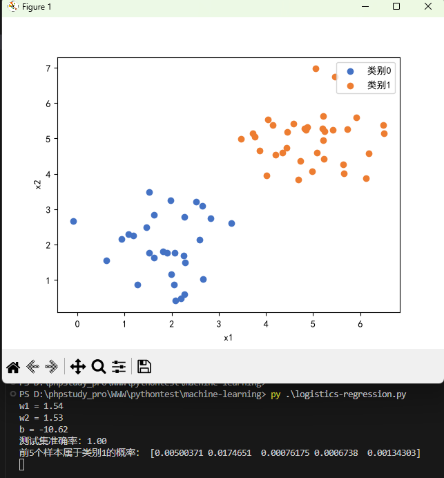
X1 = np.random.normal(loc=[2,2], scale=0.8, size=(40,2))
X2 = np.random.normal(loc=[5,5], scale=0.8, size=(40,2))
X = np.vstack([X1, X2])
y = np.hstack([np.zeros(40), np.ones(40)])

# 划分训练集、测试集
X_train, X_test, y_train, y_test = train_test_split(X, y, test_size=0.2, random_state=42)

# 训练逻辑回归
model = LogisticRegression()
model.fit(X_train, y_train)

# 输出权重和偏置
print(f"w1 = {model.coef_[0][0].item():.2f}")
print(f"w2 = {model.coef_[0][1].item():.2f}")
print(f"b = {model.intercept_.item():.2f}")

# 预测
y_pred = model.predict(X_test)
y_pred_prob = model.predict_proba(X_test)
acc = accuracy_score(y_test, y_pred)
print(f"测试集准确率：{acc:.2f}")
print("前5个样本属于类别1的概率：", y_pred_prob[:5,1])

# 绘图
plt.scatter(X_train[y_train==0,0], X_train[y_train==0,1], c="#4472c4", label="类别0")
plt.scatter(X_train[y_train==1,0], X_train[y_train==1,1], c="#ed7d31", label="类别1")
plt.legend()
plt.xlabel("x1")
plt.ylabel("x2")
plt.show()

5. 适用场景

• 二分类：是否违约、是否患病、垃圾邮件识别
• 风险评估、点击率预估
• 需要输出概率、要求可解释的业务场景

6. 常见误区

1. 逻辑回归是回归算法：名字叫回归，任务是分类。
2. 阈值固定0.5不能改：业务中可以根据召回/精确率需求调整阈值。
3. 能直接处理非线性边界：原生逻辑回归是线性分类器，非线性需要搭配多项式特征。

思考题

1. 逻辑回归为什么不用MSE，而使用交叉熵作为损失函数？
2. 如果业务希望尽量不漏掉正样本，应该调高还是调低分类阈值？